39 how to add horizontal labels in excel graph
How To Change Y-Axis Values in Excel (2 Methods) Follow these steps to switch the placement of the Y and X-axis values in an Excel chart: 1. Select the chart Navigate to the chart containing your desired data. Click anywhere on the chart to allow editing and open the "Chart Settings" tab in the toolbar. Ensure that your cursor remains in the chart area to allow for editing. 2. Open "Select Data" Make a Logarithmic Graph in Excel (semi-log and log-log) Click Insert >> Charts >> Insert Scatter (X, Y) or Bubble Chart >> Scatter with Smooth Lines and Markers. Right-click the inserted empty chart and click Select Data from the shortcut menu. In the Select Data Source dialog box, click Add in the Legend Entries (Series) area.
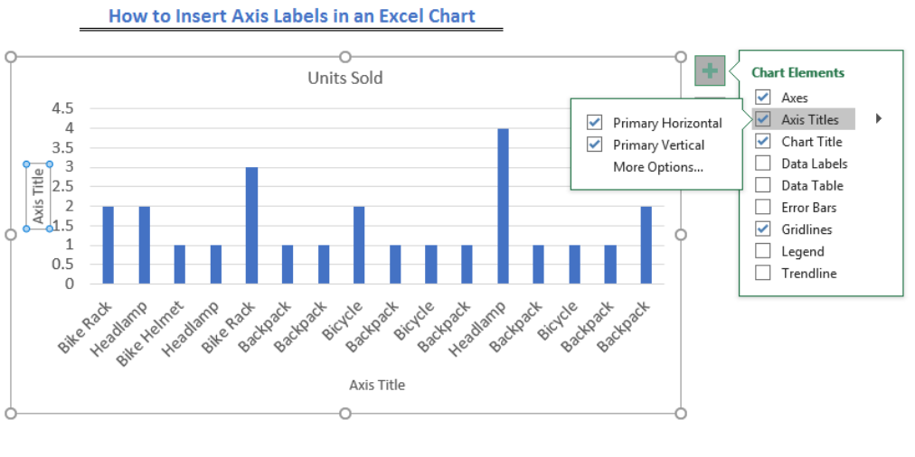
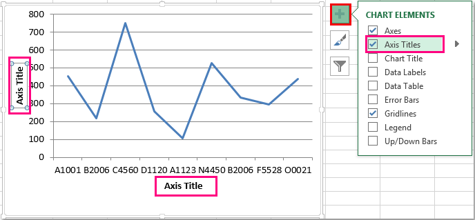
How to Add X and Y Axis Labels in Excel (2 Easy Methods) Then go to Add Chart Element and press on the Axis Titles. Moreover, select Primary Horizontal to label the horizontal axis. In short: Select graph > Chart Design > Add Chart Element > Axis Titles > Primary Horizontal. Afterward, if you have followed all steps properly, then the Axis Title option will come under the horizontal line.

How to add horizontal labels in excel graph
› 2018/09/12 › add-line-excel-graphHow to add a line in Excel graph (average line, benchmark ... Sep 12, 2018 · Draw an average line in Excel graph; Add a line to an existing Excel chart; Plot a target line with different values; How to customize the line. Display the average / target value on the line; Add a text label for the line; Change the line type; Extend the line to the edges of the graph area; How to draw an average line in Excel graph › charts › add-data-pointAdd Data Points to Existing Chart – Excel & Google Sheets Start with your Graph. Similar to Excel, create a line graph based on the first two columns (Months & Items Sold) Right click on graph; Select Data Range . 3. Select Add Series. 4. Click box for Select a Data Range. 5. Highlight new column and click OK. Final Graph with Single Data Point › add-vertical-line-excel-chartAdd vertical line to Excel chart: scatter plot, bar and line ... May 15, 2019 · In the modern versions of Excel 2013, Excel 2016 and Excel 2019, you can add a horizontal line to a chart with a few clicks, whether it's an average line, target line, benchmark, baseline or whatever. But there is still no easy way to draw a vertical line in Excel graph. However, "no easy way" does not mean no way at all.
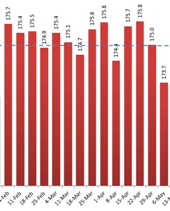
How to add horizontal labels in excel graph. How to Add Two Data Labels in Excel Chart (with Easy Steps) Table of Contents hide. Download Practice Workbook. 4 Quick Steps to Add Two Data Labels in Excel Chart. Step 1: Create a Chart to Represent Data. Step 2: Add 1st Data Label in Excel Chart. Step 3: Apply 2nd Data Label in Excel Chart. Step 4: Format Data Labels to Show Two Data Labels. Things to Remember. How to Add a Marker Line in Excel Graph (3 Suitable Examples) - ExcelDemy How to Draw a Horizontal Line in Excel Graph (2 Easy Ways) Make a Single Line Graph in Excel (A Short Way) Example 2: Add Marker Line in Scatter Plot We can plot the maximum value of datasets and mark them using error bars. We will use the MAX function to estimate the maximum value. Steps How to Change Axis Labels in Excel (3 Easy Methods) For changing the label of the Horizontal axis, follow the steps below: Firstly, right-click the category label and click Select Data > Click Edit from the Horizontal (Category) Axis Labels icon. Then, assign a new Axis label range and click OK. Now, press OK on the dialogue box. Finally, you will get your axis label changed. peltiertech.com › add-horizontal-line-to-excel-chartAdd a Horizontal Line to an Excel Chart - Peltier Tech Sep 11, 2018 · A common task is to add a horizontal line to an Excel chart. The horizontal line may reference some target value or limit, and adding the horizontal line makes it easy to see where values are above and below this reference value. Seems easy enough, but often the result is less than ideal. This tutorial shows how to add horizontal lines to ...
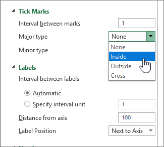
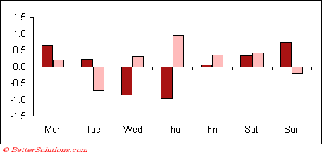
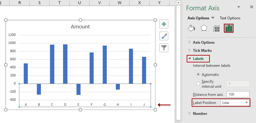
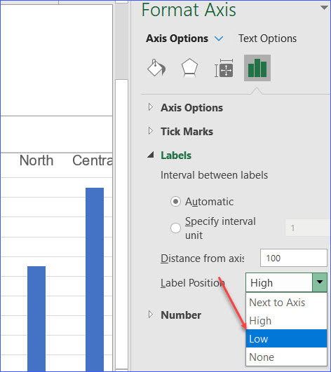
› excel › how-to-add-total-dataHow to Add Total Data Labels to the Excel Stacked Bar Chart Apr 03, 2013 · Step 4: Right click your new line chart and select “Add Data Labels” Step 5: Right click your new data labels and format them so that their label position is “Above”; also make the labels bold and increase the font size. Step 6: Right click the line, select “Format Data Series”; in the Line Color menu, select “No line” › Make-a-Bar-Graph-in-ExcelHow to Make a Bar Graph in Excel: 9 Steps (with Pictures) May 02, 2022 · Customize your graph's appearance. Once you decide on a graph format, you can use the "Design" section near the top of the Excel window to select a different template, change the colors used, or change the graph type entirely. The "Design" window only appears when your graph is selected. To select your graph, click it. How to move Excel chart axis labels to the bottom or top - Data Cornering Move Excel chart axis labels to the bottom in 2 easy steps Select horizontal axis labels and press Ctrl + 1 to open the formatting pane. Open the Labels section and choose label position " Low ". Here is the result with Excel chart axis labels at the bottom. Now it is possible to clearly evaluate the dynamics of the series and see axis labels. A Step-by-Step Guide on How to Make a Graph in Excel - Simplilearn.com For labels on the horizontal axis labels, you may select confirmed cases, deaths, recovered, and active cases, and depict them on the chart. After specifying the entries, click on OK. This will display the pie chart on your window. You can click on the icons next to the chart to add your finishing touches to it.
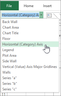
How to show percentage in Bar chart in Powerpoint - Profit claims 6. Select chart and click on Select Databutton and select Series 2 and click on Edit button under Horizontal Axis Labels and then give reference F3:F6 in Axis Label Range. Change Horizontal Axis Labels7. Right Click on bar and click on Add Data Labels Button. 8. Right Click on bar and click on Format Data Labels Button and then uncheck Value ... How to Add Axis Labels in Microsoft Excel - Appuals.com Click on the Chart Elements button (represented by a green + sign) next to the upper-right corner of the selected chart. Enable Axis Titles by checking the checkbox located directly beside the Axis Titles option. Once you do so, Excel will add labels for the primary horizontal and primary vertical axes to the chart. Horizontal axis labels on a chart - Microsoft Community If you start with Jan or January, then fill down, Excel should automatically fill in the following names. Click on the chart. Click 'Select Data' on the 'Chart Design' tab of the ribbon. Click Edit under 'Horizontal (Category) Axis Labels'. Point to the range with the months, then OK your way out. --- Kind regards, HansV Chart - how to re-arrange order of horizontal axis labels in a chart I've created a bar chart with horizontal orientation to show progress of multiple projects. I'd like the order it displayed to match my table starting from "All Projects" through "Project 11". I know how to change the order in the series but not in the axis - here is a screen shot of the simple chart and the data series but they are in the axis ...
EXCEL Charts: Column, Bar, Pie and Line
How to Rotate Axis Labels in Excel (With Example) - Statology Then click the Insert tab along the top ribbon, then click the icon called Scatter with Smooth Lines and Markers within the Charts group. The following chart will automatically appear: By default, Excel makes each label on the x-axis horizontal. However, this causes the labels to overlap in some areas and makes it difficult to read.
How to Move X Axis Labels from Bottom to Top - ExcelNotes
Excel: How to Create a Bubble Chart with Labels - Statology To add labels to the bubble chart, click anywhere on the chart and then click the green plus "+" sign in the top right corner. Then click the arrow next to Data Labels and then click More Options in the dropdown menu: In the panel that appears on the right side of the screen, check the box next to Value From Cells within the Label Options ...
Add a Horizontal Line to an Excel Chart - Peltier Tech
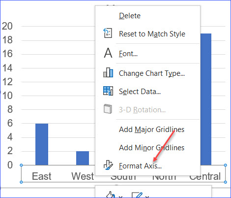
Modifying Axis Scale Labels (Microsoft Excel) - tips Follow these steps: Create your chart as you normally would. Double-click the axis you want to scale. You should see the Format Axis dialog box. (If double-clicking doesn't work, right-click the axis and choose Format Axis from the resulting Context menu.) Make sure the Number tab is displayed. (See Figure 1.)
How to create two horizontal axes on the same side ...
How to Change the X-Axis in Excel - Alphr Open the Excel file with the chart you want to adjust. Right-click the X-axis in the chart you want to change. That will allow you to edit the X-axis specifically. Then, click on Select Data. Next ...

Dynamically Label Excel Chart Series Lines • My Online ...
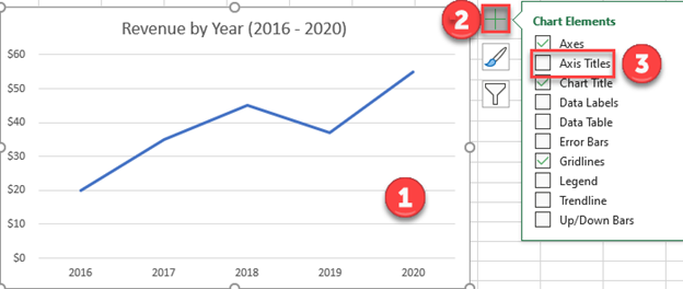
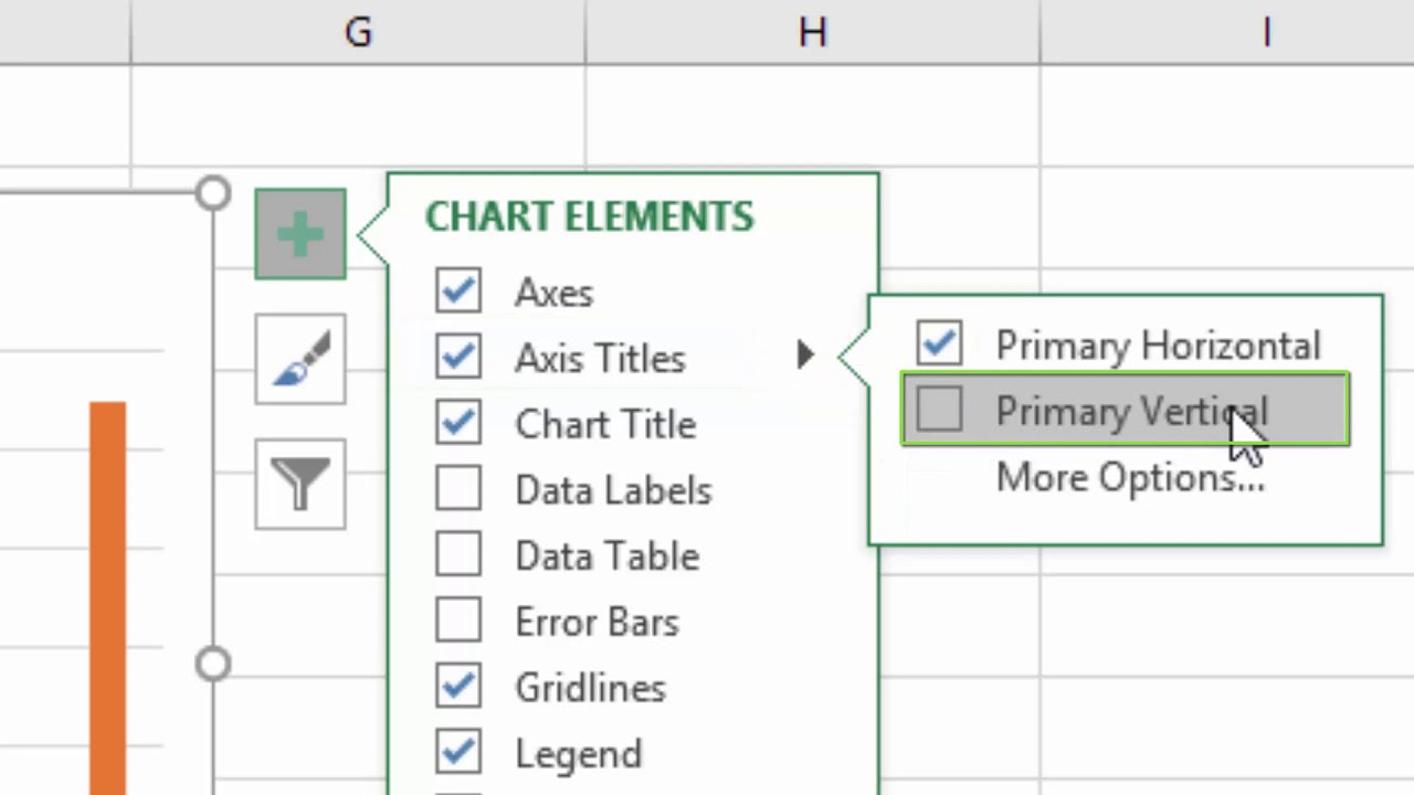
How to Add Axis Titles in a Microsoft Excel Chart - How-To Geek Select your chart and then head to the Chart Design tab that displays. Click the Add Chart Element drop-down arrow and move your cursor to Axis Titles. In the pop-out menu, select "Primary Horizontal," "Primary Vertical," or both. If you're using Excel on Windows, you can also use the Chart Elements icon on the right of the chart.
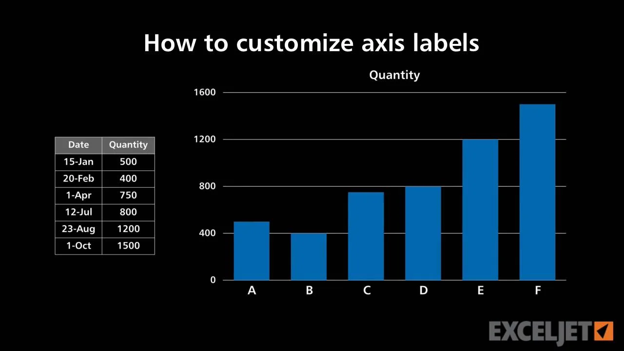
How to customize axis labels
How to add label to axis in excel chart on mac - WPS Office 1. After choosing your chart, go to the Chart Design tab that appears. Axis Titles will appear when you choose them with the drop-down arrow next to Add Chart Element. Choose Primary Horizontal, Primary Vertical, or both from the pop-out menu. 2. The Chart Elements icon is located to the right of the chart in Excel for Windows.
How to add Axis Labels (X & Y) in Excel & Google Sheets ...
excel - Add horizontal lines to plot after changing to Log scale in VBA ... I used. .Axes (xlValue).ScaleType = xlScaleLogarithmic .Axes (xlValue).LogBase = 2.7. to change the y-axis to log, however, now it looks something like this. and I want it to like something like this (this is another plot, I just want to illustrate how I want the horizontal lines). Note that the horizontal lines are only removed when I change ...
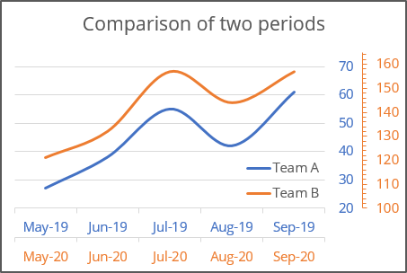
How to create two horizontal axes on the same side ...
Add axis label in excel | WPS Office Academy 1. First click so you can choose the type of chart where you want to place the axis label. 2. Now click where the chart elements button is located in the right corner of the chart. Then where the expanded menu is located, you must mark the axis titles alternative. 3.

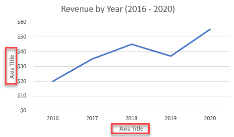
How to Add Axis Labels to a Chart in Excel - Business ...
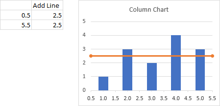
How to Add a Vertical Line to Charts in Excel - Statology This tutorial provides a step-by-step example of how to add a vertical line to the following line chart in Excel: Let's jump in! Step 1: Enter the Data. Suppose we would like to create a line chart using the following dataset in Excel: Step 2: Add Data for Vertical Line. Now suppose we would like to add a vertical line located at x = 6 on the ...
Change the display of chart axes
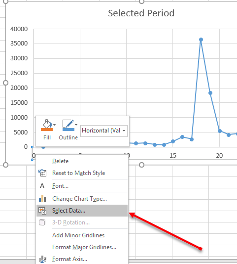
superuser.com › questions › 1484623Can't edit horizontal (catgegory) axis labels in excel Sep 20, 2019 · I'm using Excel 2013. Like in the question above, when I chose Select Data from the chart's right-click menu, I could not edit the horizontal axis labels! I got around it by first creating a 2-D column plot with my data. Next, from the chart's right-click menu: Change Chart Type. I changed it to line (or whatever you want).

How to Insert Axis Labels In An Excel Chart | Excelchat
How To Change the Scale on an Excel Graph (With Tips) Here are the basic steps involved in changing the scale on an Excel graph: 1. Determine what needs to be changed. The first step to changing the scale on your graph is determining what you'd like to change. In the example below, a book editor is making a graph that displays the total amount of sales each genre had during each month of the year.
How to I rotate data labels on a column chart so that they ...
How to format axis labels individually in Excel - SpreadsheetWeb Double-click on the axis you want to format. Double-clicking opens the right panel where you can format your axis. Open the Axis Options section if it isn't active. You can find the number formatting selection under Number section. Select Custom item in the Category list. Type your code into the Format Code box and click Add button.
Change the display of chart axes
Create A Pie Chart In Excel With and Easy Step-By-Step Guide Step 1: Select the whole dataset. Step 2: Click on the Insert tab. Step 3: Now, in the charts group, you need to click on the "Insert Pie or Doughnut Chart" option. Step 4: Click on the pie icon that is within the 2-D pie icons. These steps will add a pie chart to your Excel worksheet. You can easily figure out the approximate value of ...
How to add Axis Labels (X & Y) in Excel & Google Sheets ...
How To Add a Target Line in Excel (Using Two Different Methods) Open Excel on your device. In order to add a target line in Excel, first, open the program on your device. Either click on the Excel icon or type it into your application search bar. Once you open Excel, you can either create a new spreadsheet or edit an existing one. 2.
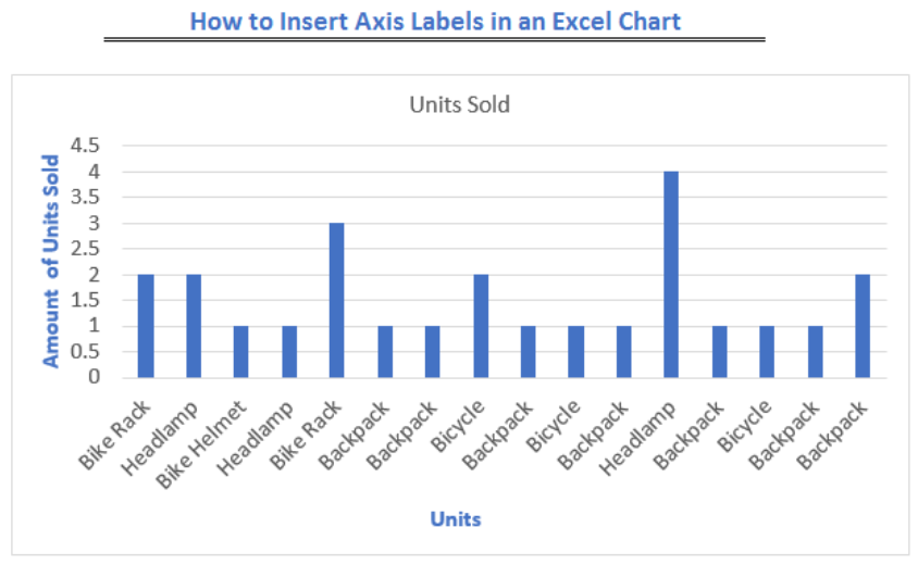
How to Insert Axis Labels In An Excel Chart | Excelchat
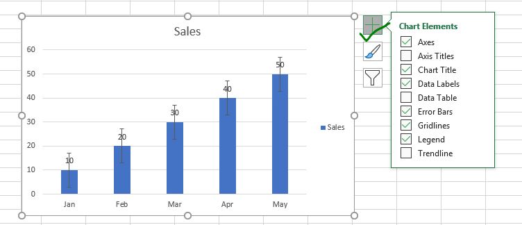
How to Add Total Values to Stacked Bar Chart in Excel Step 4: Add Total Values. Next, right click on the yellow line and click Add Data Labels. Next, double click on any of the labels. In the new panel that appears, check the button next to Above for the Label Position: Next, double click on the yellow line in the chart. In the new panel that appears, check the button next to No line:

How to label x and y axis in Microsoft excel 2016
How to add text labels on Excel scatter chart axis 3. Add dummy series to the scatter plot and add data labels. 4. Select recently added labels and press Ctrl + 1 to edit them. Add custom data labels from the column "X axis labels". Use "Values from Cells" like in this other post and remove values related to the actual dummy series. Change the label position below data points.

How to Label Axes in Excel: 6 Steps (with Pictures) - wikiHow
How to Add Secondary X Axis in Excel (with Quick Steps) Click on the arrow in the Axes option and you will find the Secondary horizontal axis. Mark the checkbox to enable and show it in the graph. 📌 Step 3: Give Axes Titles Now, to add titles in the axes, go to the chart elements again and click on the arrow in the axis titles and mark the secondary horizontal option.
Excel Charts - Move X-Axis Labels Below Negatives
› add-vertical-line-excel-chartAdd vertical line to Excel chart: scatter plot, bar and line ... May 15, 2019 · In the modern versions of Excel 2013, Excel 2016 and Excel 2019, you can add a horizontal line to a chart with a few clicks, whether it's an average line, target line, benchmark, baseline or whatever. But there is still no easy way to draw a vertical line in Excel graph. However, "no easy way" does not mean no way at all.

Excel: How to Create a Bubble Chart with Labels - Statology
› charts › add-data-pointAdd Data Points to Existing Chart – Excel & Google Sheets Start with your Graph. Similar to Excel, create a line graph based on the first two columns (Months & Items Sold) Right click on graph; Select Data Range . 3. Select Add Series. 4. Click box for Select a Data Range. 5. Highlight new column and click OK. Final Graph with Single Data Point
How to move chart X axis below negative values/zero/bottom in ...
› 2018/09/12 › add-line-excel-graphHow to add a line in Excel graph (average line, benchmark ... Sep 12, 2018 · Draw an average line in Excel graph; Add a line to an existing Excel chart; Plot a target line with different values; How to customize the line. Display the average / target value on the line; Add a text label for the line; Change the line type; Extend the line to the edges of the graph area; How to draw an average line in Excel graph
How To Add Axis Labels In Excel - BSUPERIOR

How to Add Axis Labels in Excel Charts - Step-by-Step (2022)
How to Change Horizontal Axis Labels in Excel 2010 - Solve ...
How to Move X Axis Labels from Top to Bottom - ExcelNotes
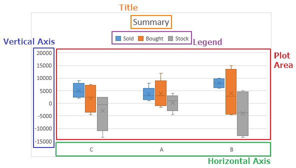
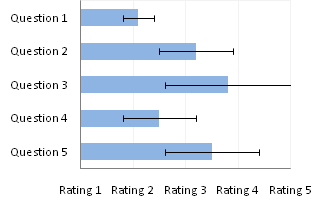
Box-and-Whisker Charts
Change Horizontal Axis Values in Excel 2016 - AbsentData
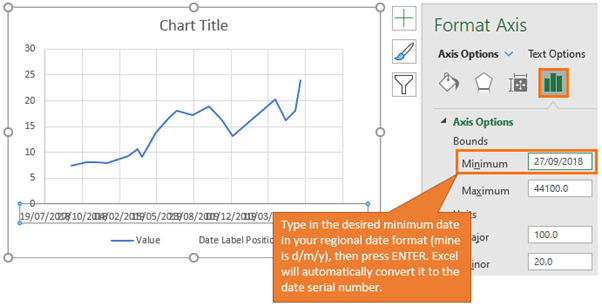
Label Specific Excel Chart Axis Dates • My Online Training Hub

Excel charts: add title, customize chart axis, legend and ...
How to Insert Axis Labels In An Excel Chart | Excelchat

Change axis labels in a chart

EXCEL Charts: Column, Bar, Pie and Line
Text Labels on a Horizontal Bar Chart in Excel - Peltier Tech

Stagger long axis labels and make one label stand out in an ...
How to add axis label to chart in Excel?

How to Add Total Data Labels to the Excel Stacked Bar Chart ...

Change axis labels in a chart

How to wrap X axis labels in a chart in Excel?
How to Add and Remove Chart Elements in Excel

Changing Axis Labels in PowerPoint 2013 for Windows
Post a Comment for "39 how to add horizontal labels in excel graph"