42 data labels excel pie chart
Edit titles or data labels in a chart - support.microsoft.com To edit the contents of a title, click the chart or axis title that you want to change. To edit the contents of a data label, click two times on the data label that you want to change. The first click selects the data labels for the whole data series, and the second click selects the individual data label. Click again to place the title or data ... Pie Chart Examples | Types of Pie Charts in Excel with Examples It is similar to Pie of the pie chart, but the only difference is that instead of a sub pie chart, a sub bar chart will be created. With this, we have completed all the 2D charts, and now we will create a 3D Pie chart. 4. 3D PIE Chart. A 3D pie chart is similar to PIE, but it has depth in addition to length and breadth.
Move data labels - support.microsoft.com Click any data label once to select all of them, or double-click a specific data label you want to move. Right-click the selection > Chart Elements > Data Labels arrow, and select the placement option you want. Different options are available for different chart types. For example, you can place data labels outside of the data points in a pie ...

Data labels excel pie chart
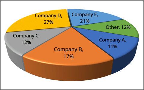
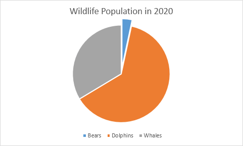
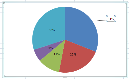
Best Types of Charts in Excel for Data Analysis, Presentation ... Apr 29, 2022 · When your data is represented in ‘percentage’ or ‘part of’, then a pie chart best meets your needs. #4 Use a pie chart to show data composition only when the pie slices are of comparable sizes. In other words, do not use a pie chart if the size of one pie slice completely dwarfs the size of the other pie slice(s): How to display leader lines in pie chart in Excel? - ExtendOffice To display leader lines in pie chart, you just need to check an option then drag the labels out. 1. Click at the chart, and right click to select Format Data Labels from context menu. 2. In the popping Format Data Labels dialog/pane, check Show Leader Lines in the Label Options section. See screenshot: How to Make a PIE Chart in Excel (Easy Step-by-Step Guide) Creating a Pie Chart in Excel. To create a Pie chart in Excel, you need to have your data structured as shown below. The description of the pie slices should be in the left column and the data for each slice should be in the right column. Once you have the data in place, below are the steps to create a Pie chart in Excel: Select the entire dataset
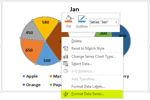
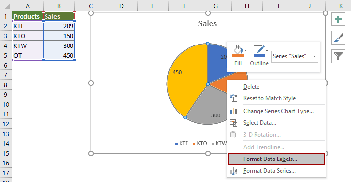
Data labels excel pie chart. excel - Pie Chart VBA DataLabel Formatting - Stack Overflow Pie Chart VBA DataLabel Formatting. Ask Question Asked 3 years, 11 months ago. ... Excel VBA to fill pie chart colors from cells with conditional formatting. 0. ... Formatting chart data labels with VBA. 1. Excel VBA Updating Chart Series. 0. Formatting charts in a chart group. How to Make a Pie Chart in Excel & Add Rich Data Labels to ... Sep 08, 2022 · In this article, we are going to see a detailed description of how to make a pie chart in excel. One can easily create a pie chart and add rich data labels, to one’s pie chart in Excel. So, let’s see how to effectively use a pie chart and add rich data labels to your chart, in order to present data, using a simple tennis related example. Pie Chart in Excel | How to Create Pie Chart - EDUCBA Step 1: Do not select the data; rather, place a cursor outside the data and insert one PIE CHART. Go to the Insert tab and click on a PIE. Step 2: once you click on a 2-D Pie chart, it will insert the blank chart as shown in the below image. Step 3: Right-click on the chart and choose Select Data. Step 4: once you click on Select Data, it will ... Create a Pie Chart in Excel (Easy Tutorial) 6. Create the pie chart (repeat steps 2-3). 7. Click the legend at the bottom and press Delete. 8. Select the pie chart. 9. Click the + button on the right side of the chart and click the check box next to Data Labels. 10. Click the paintbrush icon on the right side of the chart and change the color scheme of the pie chart. Result: 11.
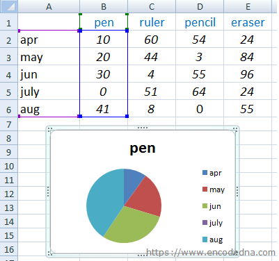
How to Make a Pie Chart with Multiple Data in Excel (2 Ways) - ExcelDemy Steps: First, select the entire data set and go to the Insert tab from the ribbon. After that, choose Insert Pie and Doughnut Chart from the Charts group. Afterward, click on the 2nd Pie Chart among the 2-D Pie as marked on the following picture. Now, Excel will instantly create a Pie of Pie Chart in your worksheet. Add or remove data labels in a chart - support.microsoft.com For example, in the pie chart below, without the data labels it would be difficult to tell that coffee was 38% of total sales. Depending on what you want to highlight on a chart, you can add labels to one series, all the series (the whole chart), or one data point. ... You can add data labels to show the data point values from the Excel sheet ... How to Create a Pie Chart in Excel | Smartsheet Aug 27, 2018 · To create a pie chart in Excel 2016, add your data set to a worksheet and highlight it. Then click the Insert tab, and click the dropdown menu next to the image of a pie chart. Select the chart type you want to use and the chosen chart will appear on the worksheet with the data you selected. Create A Pie Chart In Excel With and Easy Step-By-Step Guide Sep 22, 2022 · Creating A Pie Chart In Excel. If you wish to create a pie chart in Excel, then you need to have all your data structured as we have shown below. The description of the slices of the pie should always be on the left side and on the right side; you should enter the data for every slice.
How to add data labels in excel to graph or chart (Step-by-Step) 1. Select a data series or a graph. After picking the series, click the data point you want to label. 2. Click Add Chart Element Chart Elements button > Data Labels in the upper right corner, close to the chart. 3. Click the arrow and select an option to modify the location. 4. Change the format of data labels in a chart To get there, after adding your data labels, select the data label to format, and then click Chart Elements > Data Labels > More Options. To go to the appropriate area, click one of the four icons ( Fill & Line, Effects, Size & Properties ( Layout & Properties in Outlook or Word), or Label Options) shown here. Pie Chart in Excel - Inserting, Formatting, Filters, Data Labels The total of percentages of the data point in the pie chart would be 100% in all cases. Consequently, we can add Data Labels on the pie chart to show the numerical values of the data points. We can use Pie Charts to represent: ratio of population of male and female of a country. proportion of online/offline payment modes of a local car rental ... How to Create and Format a Pie Chart in Excel - Lifewire To create a pie chart, highlight the data in cells A3 to B6 and follow these directions: On the ribbon, go to the Insert tab. Select Insert Pie Chart to display the available pie chart types. Hover over a chart type to read a description of the chart and to preview the pie chart. Choose a chart type.
Microsoft Excel Tutorials: Add Data Labels to a Pie Chart
Excel Pie Chart - How to Create & Customize? (Top 5 Types) The steps to add percentages to the Pie Chart are: Step 1: Click on the Pie Chart > click the ' + ' icon > check/tick the " Data Labels " checkbox in the " Chart Element " box > select the " Data Labels " right arrow > select the " More Options… ", as shown below. Step 2: The Format Data Labels pane opens.

Chart Data Labels in PowerPoint 2013 for Windows
Add or remove data labels in a chart - support.microsoft.com Data labels make a chart easier to understand because they show details about a data series or its individual data points. For example, in the pie chart below, without the data labels it would be difficult to tell that coffee was 38% of total sales. Depending on what you want to highlight on a chart, you can add labels to one series, all the ...

Add data labels and callouts to charts in Excel 365 ...
How to add data labels from different column in an Excel chart? Please do as follows: 1. Right click the data series in the chart, and select Add Data Labels > Add Data Labels from the context menu to add data labels. 2. Right click the data series, and select Format Data Labels from the context menu. 3.

How to Data Labels in a Pie chart in Excel 2010
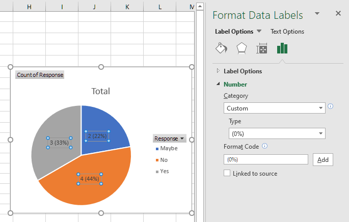
How to hide zero data labels in chart in Excel? - ExtendOffice If you want to hide zero data labels in chart, please do as follow: 1. Right click at one of the data labels, and select Format Data Labels from the context menu. See screenshot: 2. In the Format Data Labels dialog, Click Number in left pane, then select Custom from the Category list box, and type #"" into the Format Code text box, and click Add button to add it to Type list box.

How to make a pie chart in Excel
How to insert data labels to a Pie chart in Excel 2013 - YouTube This video will show you the simple steps to insert Data Labels in a pie chart in Microsoft® Excel 2013. Content in this video is provided on an "as is" basi...

How to Create a Pie Chart in Excel | Smartsheet
Creating Pie Chart and Adding/Formatting Data Labels (Excel) Creating Pie Chart and Adding/Formatting Data Labels (Excel)

Change the format of data labels in a chart
How to Make a PIE Chart in Excel (Easy Step-by-Step Guide) Creating a Pie Chart in Excel. To create a Pie chart in Excel, you need to have your data structured as shown below. The description of the pie slices should be in the left column and the data for each slice should be in the right column. Once you have the data in place, below are the steps to create a Pie chart in Excel: Select the entire dataset
Excel 3-D Pie charts - Microsoft Excel 365
How to display leader lines in pie chart in Excel? - ExtendOffice To display leader lines in pie chart, you just need to check an option then drag the labels out. 1. Click at the chart, and right click to select Format Data Labels from context menu. 2. In the popping Format Data Labels dialog/pane, check Show Leader Lines in the Label Options section. See screenshot:

Create Outstanding Pie Charts in Excel | Pryor Learning
Best Types of Charts in Excel for Data Analysis, Presentation ... Apr 29, 2022 · When your data is represented in ‘percentage’ or ‘part of’, then a pie chart best meets your needs. #4 Use a pie chart to show data composition only when the pie slices are of comparable sizes. In other words, do not use a pie chart if the size of one pie slice completely dwarfs the size of the other pie slice(s):
Excel custom pie chart labels - Microsoft Community

Optimally positioning pie chart data labels in Excel with VBA ...
How to Create a Pie Chart in Excel using Worksheet Data

How to make doughnut chart with outside end labels - Simple ...

Office: Display Data Labels in a Pie Chart

Change the format of data labels in a chart

How to Change Excel Chart Data Labels to Custom Values?

How to make a pie chart in Excel

Change color of data label placed, using the 'best fit ...

How to Make Pie Chart with Labels both Inside and Outside ...

Custom data labels in a chart

How to Create a Pie Chart in Excel | Smartsheet

How to Make Pie Chart with Labels both Inside and Outside ...

How to Create a Pie Chart in Excel | Smartsheet
Excel Doughnut chart with leader lines – teylyn

Add or remove data labels in a chart

PowerPoint Data Labels on Pie of Pie Charts | MrExcel Message ...
KB209780: Data labels overlap when exporting a pie graph in a ...

Creating Pie Chart and Adding/Formatting Data Labels (Excel)

How to Make a Pie Chart in Excel
KB209780: Data labels overlap when exporting a pie graph in a ...
Create a Pie Chart in Excel (Easy Tutorial)
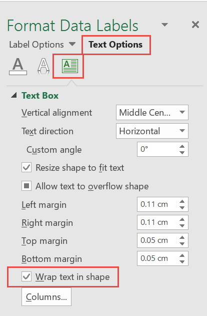
How to fix wrapped data labels in a pie chart - Excel Tips ...

Change the format of data labels in a chart

excel - Prevent overlapping of data labels in pie chart ...
Pie Charts in Excel - How to Make with Step by Step Examples

How-to Add Label Leader Lines to an Excel Pie Chart - Excel ...
How to show percentage in pie chart in Excel?

How to fix wrapped data labels in a pie chart | Sage Intelligence

EXCEL Charts: Column, Bar, Pie and Line
How-to Add Label Leader Lines to an Excel Pie Chart - Excel ...

How to show percentage in pie chart in Excel?

Pie Chart – Excel Tutorial
Post a Comment for "42 data labels excel pie chart"